Loan Repayment Prediction
A LightGBM Model to identify borrowers who are most likely to repay a loan,thus resulting in a profitable bank.

Business Problem
The two most critical questions in the lending industry are: 1) How risky is the borrower? 2) Given the borrower’s risk, should we lend him/her? The answer to the first question determines the interest rate the borrower would have. Interest rate measures among other things (such as time value of money) the riskness of the borrower, i.e. the riskier the borrower, the higher the interest rate.
Investors (lenders) provide loans to borrowers in exchange for the promise of repayment with interest. That means the lender only makes profit (interest) if the borrower pays off the loan. However, if he/she doesn’t repay the loan, then the lender loses money.
Our Goal is to understand the loan business of the bank.It wants to identify who would be the right target for the loans. The data contains both customers who have been given loans and those who haven’t yet received loans. The aim is to identify of the customers who haven’t been granted a loan which are more likely to repay the loan and provide loans to them.
Data Set
- Borrower_table - informtion about the borrowers such as age, salary, checking/savings amount and previous credit history.
- Loan_table – loan details such as repayment history, loan purpose.
Roadmap
- Dataset missing value, outlier analysis
- Data Transformation
- Data Exploration for Insights
- Data Preparation for Model Building
- Model Build to maximize profit
- Model Selection
- Recommendations based on target audience
import numpy as np
import pandas as pd


from sklearn.metrics import auc, roc_curve,roc_auc_score, classification_report,accuracy_score
from sklearn.metrics import roc_curve
from sklearn.ensemble import RandomForestClassifier, GradientBoostingClassifier
from sklearn.model_selection import train_test_split
from sklearn.preprocessing import LabelEncoder
import matplotlib.pyplot as plt
import seaborn as sns

plt.style.use('ggplot')
%matplotlib inline
import lightgbm as lgb
Data Loading
Loan Table:
- Dataset contains 101100 unique loans and has 5 features including loan granted and loan repaid.
- Loan Repaid has 3 values: 0,1,NaN
- Definition of Loan Repaid:
Loan Granted and Repaid then repaid is 1
Loan Granted and Not Repaid then repaid is 0
Loan Not Granted then Repaid is NaN
loan = pd.read_csv('loan_table.csv',parse_dates =[ 'date'])
loan.head()
| loan_id | loan_purpose | date | loan_granted | loan_repaid | |
|---|---|---|---|---|---|
| 0 | 19454 | investment | 2012-03-15 | 0 | NaN |
| 1 | 496811 | investment | 2012-01-17 | 0 | NaN |
| 2 | 929493 | other | 2012-02-09 | 0 | NaN |
| 3 | 580653 | other | 2012-06-27 | 1 | 1.0 |
| 4 | 172419 | business | 2012-05-21 | 1 | 0.0 |
loan.shape
(101100, 5)
len(loan.loan_id.unique())
101100
loan.isnull().sum()
loan_id             0
loan_purpose        0
date                0
loan_granted        0
loan_repaid     53446
dtype: int64
loan[(loan.loan_granted == 1) & (loan.loan_repaid.isnull())]
| loan_id | loan_purpose | date | loan_granted | loan_repaid |
|---|
Borrower Table:
Dataset has loan id which is foreign key to loans table.
It has 101100 obs with 12 features related to the borrower.
A few columns have missing values. Currently Repaying other loans will be Nan if the borrower has never applied for a loan before.
borrower = pd.read_csv('borrower_table.csv')
borrower.head()
| loan_id | is_first_loan | fully_repaid_previous_loans | currently_repaying_other_loans | total_credit_card_limit | avg_percentage_credit_card_limit_used_last_year | saving_amount | checking_amount | is_employed | yearly_salary | age | dependent_number | |
|---|---|---|---|---|---|---|---|---|---|---|---|---|
| 0 | 289774 | 1 | NaN | NaN | 8000 | 0.49 | 3285 | 1073 | 0 | 0 | 47 | 3 |
| 1 | 482590 | 0 | 1.0 | 0.0 | 4500 | 1.03 | 636 | 5299 | 1 | 13500 | 33 | 1 |
| 2 | 135565 | 1 | NaN | NaN | 6900 | 0.82 | 2085 | 3422 | 1 | 24500 | 38 | 8 |
| 3 | 207797 | 0 | 1.0 | 0.0 | 1200 | 0.82 | 358 | 3388 | 0 | 0 | 24 | 1 |
| 4 | 828078 | 0 | 0.0 | 0.0 | 6900 | 0.80 | 2138 | 4282 | 1 | 18100 | 36 | 1 |
borrower.shape
(101100, 12)
len(borrower.loan_id.unique())
101100
borrower.info()
<class 'pandas.core.frame.DataFrame'>
RangeIndex: 101100 entries, 0 to 101099
Data columns (total 12 columns):
 #   Column                                           Non-Null Count   Dtype
---  ------                                           --------------   -----
 0   loan_id                                          101100 non-null  int64
 1   is_first_loan                                    101100 non-null  int64
 2   fully_repaid_previous_loans                      46153 non-null   float64
 3   currently_repaying_other_loans                   46153 non-null   float64
 4   total_credit_card_limit                          101100 non-null  int64
 5   avg_percentage_credit_card_limit_used_last_year  94128 non-null   float64
 6   saving_amount                                    101100 non-null  int64
 7   checking_amount                                  101100 non-null  int64
 8   is_employed                                      101100 non-null  int64
 9   yearly_salary                                    101100 non-null  int64
 10  age                                              101100 non-null  int64
 11  dependent_number                                 101100 non-null  int64
dtypes: float64(3), int64(9)
memory usage: 9.3 MB
borrower.isnull().sum()
loan_id                                                0
is_first_loan                                          0
fully_repaid_previous_loans                        54947
currently_repaying_other_loans                     54947
total_credit_card_limit                                0
avg_percentage_credit_card_limit_used_last_year     6972
saving_amount                                          0
checking_amount                                        0
is_employed                                            0
yearly_salary                                          0
age                                                    0
dependent_number                                       0
dtype: int64
borrower.describe()
| loan_id | is_first_loan | fully_repaid_previous_loans | currently_repaying_other_loans | total_credit_card_limit | avg_percentage_credit_card_limit_used_last_year | saving_amount | checking_amount | is_employed | yearly_salary | age | dependent_number | |
|---|---|---|---|---|---|---|---|---|---|---|---|---|
| count | 101100.000000 | 101100.000000 | 46153.000000 | 46153.000000 | 101100.000000 | 94128.000000 | 101100.000000 | 101100.000000 | 101100.000000 | 101100.000000 | 101100.000000 | 101100.000000 |
| mean | 499666.826726 | 0.543492 | 0.899291 | 0.364332 | 4112.743818 | 0.724140 | 1799.617616 | 3177.150821 | 0.658675 | 21020.727992 | 41.491632 | 3.864748 |
| std | 288662.006929 | 0.498107 | 0.300946 | 0.481247 | 2129.121462 | 0.186483 | 1400.545141 | 2044.448155 | 0.474157 | 18937.581415 | 12.825570 | 2.635491 |
| min | 30.000000 | 0.000000 | 0.000000 | 0.000000 | 0.000000 | 0.000000 | 0.000000 | 0.000000 | 0.000000 | 0.000000 | 18.000000 | 0.000000 |
| 25% | 250333.750000 | 0.000000 | 1.000000 | 0.000000 | 2700.000000 | 0.600000 | 834.000000 | 1706.000000 | 0.000000 | 0.000000 | 32.000000 | 2.000000 |
| 50% | 499885.000000 | 1.000000 | 1.000000 | 0.000000 | 4100.000000 | 0.730000 | 1339.000000 | 2673.000000 | 1.000000 | 21500.000000 | 41.000000 | 3.000000 |
| 75% | 749706.250000 | 1.000000 | 1.000000 | 1.000000 | 5500.000000 | 0.860000 | 2409.000000 | 4241.000000 | 1.000000 | 35300.000000 | 50.000000 | 6.000000 |
| max | 999987.000000 | 1.000000 | 1.000000 | 1.000000 | 13500.000000 | 1.090000 | 10641.000000 | 13906.000000 | 1.000000 | 97200.000000 | 79.000000 | 8.000000 |
Data Merging
Combine Loan and Borrower information to get a full dataset which can be used for analysis.
full_data = pd.merge(left = borrower, right = loan, on = 'loan_id',how = 'left')
full_data.head()
| loan_id | is_first_loan | fully_repaid_previous_loans | currently_repaying_other_loans | total_credit_card_limit | avg_percentage_credit_card_limit_used_last_year | saving_amount | checking_amount | is_employed | yearly_salary | age | dependent_number | loan_purpose | date | loan_granted | loan_repaid | |
|---|---|---|---|---|---|---|---|---|---|---|---|---|---|---|---|---|
| 0 | 289774 | 1 | NaN | NaN | 8000 | 0.49 | 3285 | 1073 | 0 | 0 | 47 | 3 | business | 2012-01-31 | 0 | NaN |
| 1 | 482590 | 0 | 1.0 | 0.0 | 4500 | 1.03 | 636 | 5299 | 1 | 13500 | 33 | 1 | investment | 2012-11-02 | 0 | NaN |
| 2 | 135565 | 1 | NaN | NaN | 6900 | 0.82 | 2085 | 3422 | 1 | 24500 | 38 | 8 | other | 2012-07-16 | 1 | 1.0 |
| 3 | 207797 | 0 | 1.0 | 0.0 | 1200 | 0.82 | 358 | 3388 | 0 | 0 | 24 | 1 | investment | 2012-06-05 | 0 | NaN |
| 4 | 828078 | 0 | 0.0 | 0.0 | 6900 | 0.80 | 2138 | 4282 | 1 | 18100 | 36 | 1 | emergency_funds | 2012-11-28 | 0 | NaN |
full_data.shape
(101100, 16)
Total 47,654 loans were granted which is 47% of the total loans and 53% were not granted.
grant = len(full_data[full_data['loan_granted'] == 1])
no_grant = len(full_data[full_data['loan_granted'] == 0])
print('Total Loans Granted: {}'.format(grant))
print('Total Loans Not Granted: {}'.format(no_grant))
Total Loans Granted: 47654
Total Loans Not Granted: 53446
Filter the dataset to include only the loans which were granted. This leaves us with 47654 observations.
data = full_data[full_data['loan_granted'] == 1]
len(data)
47654
data.head()
| loan_id | is_first_loan | fully_repaid_previous_loans | currently_repaying_other_loans | total_credit_card_limit | avg_percentage_credit_card_limit_used_last_year | saving_amount | checking_amount | is_employed | yearly_salary | age | dependent_number | loan_purpose | date | loan_granted | loan_repaid | |
|---|---|---|---|---|---|---|---|---|---|---|---|---|---|---|---|---|
| 2 | 135565 | 1 | NaN | NaN | 6900 | 0.82 | 2085 | 3422 | 1 | 24500 | 38 | 8 | other | 2012-07-16 | 1 | 1.0 |
| 5 | 423171 | 1 | NaN | NaN | 6100 | 0.53 | 6163 | 5298 | 1 | 29500 | 24 | 1 | other | 2012-11-07 | 1 | 1.0 |
| 7 | 200139 | 1 | NaN | NaN | 4000 | 0.57 | 602 | 2757 | 1 | 31700 | 36 | 8 | business | 2012-09-19 | 1 | 0.0 |
| 8 | 991294 | 0 | 1.0 | 0.0 | 7000 | 0.52 | 2575 | 2917 | 1 | 58900 | 33 | 3 | emergency_funds | 2012-12-04 | 1 | 1.0 |
| 9 | 875332 | 0 | 1.0 | 0.0 | 4300 | 0.83 | 722 | 892 | 1 | 5400 | 32 | 7 | business | 2012-01-20 | 1 | 1.0 |
Data Quality Analysis
- We see that a few columns such as currently repaying previous loans has large number of nulls.
- After closer examination we see currently repaying previous loans and fully repaid previous loans is null for only first loan which makes sense since the borrower is applying for a loan for the first time.
data.info()
<class 'pandas.core.frame.DataFrame'>
Int64Index: 47654 entries, 2 to 101099
Data columns (total 16 columns):
 #   Column                                           Non-Null Count  Dtype
---  ------                                           --------------  -----
 0   loan_id                                          47654 non-null  int64
 1   is_first_loan                                    47654 non-null  int64
 2   fully_repaid_previous_loans                      21865 non-null  float64
 3   currently_repaying_other_loans                   21865 non-null  float64
 4   total_credit_card_limit                          47654 non-null  int64
 5   avg_percentage_credit_card_limit_used_last_year  46751 non-null  float64
 6   saving_amount                                    47654 non-null  int64
 7   checking_amount                                  47654 non-null  int64
 8   is_employed                                      47654 non-null  int64
 9   yearly_salary                                    47654 non-null  int64
 10  age                                              47654 non-null  int64
 11  dependent_number                                 47654 non-null  int64
 12  loan_purpose                                     47654 non-null  object
 13  date                                             47654 non-null  datetime64[ns]
 14  loan_granted                                     47654 non-null  int64
 15  loan_repaid                                      47654 non-null  float64
dtypes: datetime64[ns](1), float64(4), int64(10), object(1)
memory usage: 6.2+ MB
data.isnull().sum()
loan_id                                                0
is_first_loan                                          0
fully_repaid_previous_loans                        25789
currently_repaying_other_loans                     25789
total_credit_card_limit                                0
avg_percentage_credit_card_limit_used_last_year      903
saving_amount                                          0
checking_amount                                        0
is_employed                                            0
yearly_salary                                          0
age                                                    0
dependent_number                                       0
loan_purpose                                           0
date                                                   0
loan_granted                                           0
loan_repaid                                            0
dtype: int64
#Data quality check
data[(data.is_first_loan == 1 ) & (data.fully_repaid_previous_loans == 1.0)]
| loan_id | is_first_loan | fully_repaid_previous_loans | currently_repaying_other_loans | total_credit_card_limit | avg_percentage_credit_card_limit_used_last_year | saving_amount | checking_amount | is_employed | yearly_salary | age | dependent_number | loan_purpose | date | loan_granted | loan_repaid |
|---|
data[(data.is_first_loan == 1 ) & (data.currently_repaying_other_loans == 1.0)]
| loan_id | is_first_loan | fully_repaid_previous_loans | currently_repaying_other_loans | total_credit_card_limit | avg_percentage_credit_card_limit_used_last_year | saving_amount | checking_amount | is_employed | yearly_salary | age | dependent_number | loan_purpose | date | loan_granted | loan_repaid |
|---|
A simple initial data investigation can tell us how many loans were granted and how many were actually repaid
- Total 47654 Loan were granted
- Out of which 64% of the loans were repaid and 36% were unpaid.
tot_loans = len(data)
tot_loans_rep = len(data[data['loan_repaid'] == 1.0])
tot_loan_norep = len(data[data['loan_repaid'] == 0.0])
print('Total Loans Granted: {}'.format(tot_loans))
print('Total Loans Repaid: {}'.format(tot_loans_rep))
print('Total Loans Not Repaid: {}'.format(tot_loan_norep))
Total Loans Granted: 47654
Total Loans Repaid: 30706
Total Loans Not Repaid: 16948
Data Exploration(EDA)
We will begin by extracting some date features to better understand our data.
# parse date information and extract month, week, and dayofweek information
data['month'] = data['date'].apply(lambda x: x.month)
data['week'] = data['date'].apply(lambda x: x.week)
data['dayofweek'] = data['date'].apply(lambda x: x.dayofweek)
<ipython-input-247-a568e6d2ef8a>:2: SettingWithCopyWarning:
A value is trying to be set on a copy of a slice from a DataFrame.
Try using .loc[row_indexer,col_indexer] = value instead

See the caveats in the documentation: https://pandas.pydata.org/pandas-docs/stable/user_guide/indexing.html#returning-a-view-versus-a-copy
  data['month'] = data['date'].apply(lambda x: x.month)
<ipython-input-247-a568e6d2ef8a>:3: SettingWithCopyWarning:
A value is trying to be set on a copy of a slice from a DataFrame.
Try using .loc[row_indexer,col_indexer] = value instead

See the caveats in the documentation: https://pandas.pydata.org/pandas-docs/stable/user_guide/indexing.html#returning-a-view-versus-a-copy
  data['week'] = data['date'].apply(lambda x: x.week)
<ipython-input-247-a568e6d2ef8a>:4: SettingWithCopyWarning:
A value is trying to be set on a copy of a slice from a DataFrame.
Try using .loc[row_indexer,col_indexer] = value instead

See the caveats in the documentation: https://pandas.pydata.org/pandas-docs/stable/user_guide/indexing.html#returning-a-view-versus-a-copy
  data['dayofweek'] = data['date'].apply(lambda x: x.dayofweek)
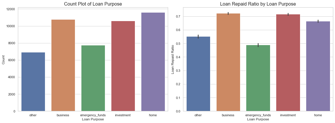
Loan Repayment Rate by Loan Purpose
Results:
- A lot of the borrowers apply for a loan when purchasing a house, or for business and investment purposes.
- Business and Investment have highest re-payment rate whereas Emergency funds have the lowest rate.
#Visualization of loan purpose
sns.set(style="whitegrid", color_codes=True)
fig, ax = plt.subplots(nrows=1, ncols=2, figsize=(16, 6))
sns.countplot(x='loan_purpose', data=data, ax=ax[0])
ax[0].set_xlabel('Loan Purpose', fontsize=12)
ax[0].set_ylabel('Count', fontsize=12)
ax[0].set_title('Count Plot of Loan Purpose', fontsize=16)

sns.barplot(x='loan_purpose', y='loan_repaid', data=data, ax=ax[1])
ax[1].set_xlabel('Loan Purpose', fontsize=12)
ax[1].set_ylabel('Loan Repaid Ratio', fontsize=12)
ax[1].set_title('Loan Repaid Ratio by Loan Purpose', fontsize=16)
plt.tight_layout()
plt.show()
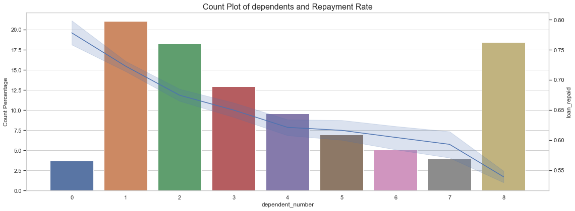
Loan Repayment Rate by Number of dependents
Results:
- My inital assumption was higher the number of dependents, lower the repayment rate. More dependents might lead to more expenses and lesser savings to repay the loan. This assumption was validated by the data.
- Loan Repayment rate is highest when number of dependents is 0 or 1 and it is inversely proportional to number of dependents.
- Just over 2.5% loans are granted to people with zero dependents but more than 17.5% are granted to people with 8 dependents.
#Dependent number

fig, ax = plt.subplots(nrows=1, ncols=1, figsize=(16, 6))
sns.barplot(x="dependent_number", y="dependent_number", data=data, estimator=lambda x: len(x) / len(data) * 100,ax = ax)
ax.set_xlabel('dependent_number', fontsize=12)
ax.set_ylabel('Count Percentage', fontsize=12)
ax.set_title('Count Plot of dependents and Repayment Rate', fontsize=16)
ax2 = ax.twinx()
sns.lineplot(x='dependent_number', y='loan_repaid', data=data, ax=ax2)
ax2.grid(False)
plt.tight_layout()
plt.show()
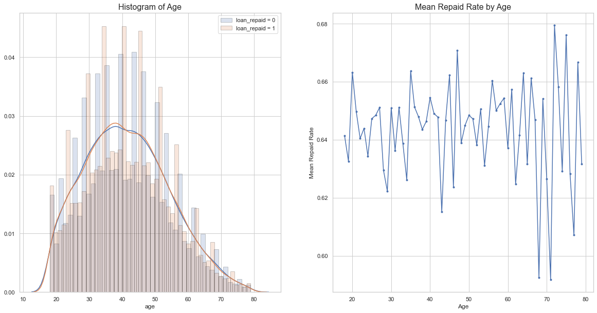
Loan Repayment Rate by Age
Results:
- A lot of the borrowers applying for the loan are between 30-55 years of age.
- Loan Repayment rate fluctuates with age.
#Age
grouped_age = data[['age', 'loan_repaid']].groupby('age')
grouped_age
mean_age = grouped_age.mean().reset_index()
fig, ax = plt.subplots(nrows=1, ncols=2, figsize=(20, 10))
hist_kws={'histtype': 'bar', 'edgecolor':'black', 'alpha': 0.2}
sns.distplot(data[data['loan_repaid'] == 0]['age'],
             label='loan_repaid = 0', ax=ax[0], hist_kws=hist_kws)
sns.distplot(data[data['loan_repaid'] == 1]['age'],
             label='loan_repaid = 1', ax=ax[0], hist_kws=hist_kws)
ax[0].set_title('Histogram of Age', fontsize=16)
ax[0].legend()
ax[1].plot(mean_age['age'], mean_age['loan_repaid'], '.-')
ax[1].set_title('Mean Repaid Rate by Age', fontsize=16)
ax[1].set_xlabel('Age')
ax[1].set_ylabel('Mean Repaid Rate')
ax[1].grid(True)
plt.show()
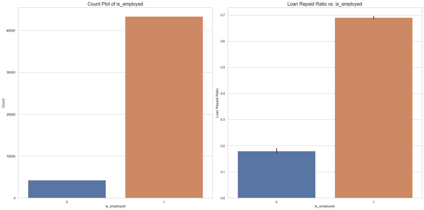
Loan Repayment Rate by Employment status
Results:
- A lot of the borrowers who were granted the loan are employed and are able to repay the loan.
- Repayment Rate among the ones who are unemployed is just 18%.
len(data[(data.is_employed == 0) & (data.loan_repaid == 1)])/len(data[data.is_employed == 0])
0.17942750756341633
#is_employed
fig, ax = plt.subplots(nrows=1, ncols=2, figsize=(20, 10))
sns.countplot(x='is_employed', data=data, ax=ax[0])
ax[0].set_xlabel('is_employed', fontsize=12)
ax[0].set_ylabel('Count', fontsize=12)
ax[0].set_title('Count Plot of is_employed', fontsize=16)

sns.barplot(x='is_employed', y='loan_repaid', data=data, ax=ax[1])
ax[1].set_xlabel('is_employed', fontsize=12)
ax[1].set_ylabel('Loan Repaid Ratio', fontsize=12)
ax[1].set_title('Loan Repaid Ratio vs. is_employed', fontsize=16)
plt.tight_layout()
plt.show()
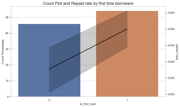
Loan Repayment Rate among first time loans
Results:
- A lot of the borrowers who were granted a loan are first time borrowers.
- More than 50% loans are granted to first-time borrowers who have a repayment rate of around 65%.
- Repayment Rate is more than 60% for both first and non-first timers.
#is_first_loan


fig, ax = plt.subplots(nrows=1, ncols=1, figsize=(10, 6))
sns.barplot(x="is_first_loan", y="is_first_loan", data=data, estimator=lambda x: len(x) / len(data) * 100,ax = ax)
ax.set_xlabel('is_first_loan', fontsize=12)
ax.set_ylabel('Count Percentage', fontsize=12)
ax.set_title('Count Plot and Repaid rate by first time borrowers', fontsize=16)
ax2 = ax.twinx()
sns.lineplot(x='is_first_loan', y='loan_repaid', data=data, color = "black",lw = 2,markers=True,ax=ax2)
ax2.grid(False)
plt.tight_layout()
plt.show()
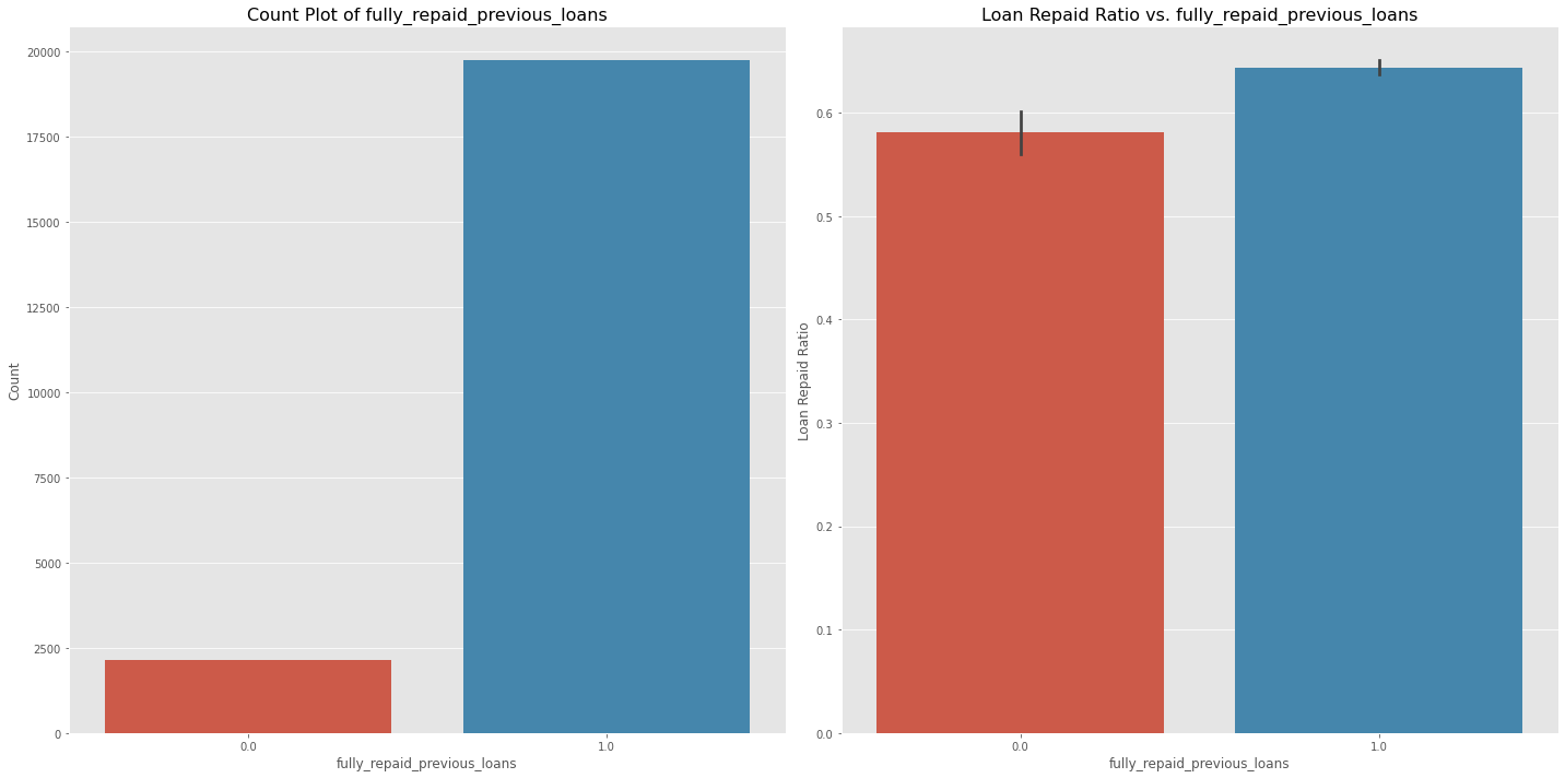
Loan Repayment Rate by Previous Loan History
Results:
- Not a lot of loans were granted to people who defaulted on their previous loans.
- Surprisingly, Repayment rate is above 55% for those who did not pay their previous loans.
#fully_repaid_previous_loans
fig, ax = plt.subplots(nrows=1, ncols=2, figsize=(20, 10))
sns.countplot(x='fully_repaid_previous_loans', data=data, ax=ax[0])
ax[0].set_xlabel('fully_repaid_previous_loans', fontsize=12)
ax[0].set_ylabel('Count', fontsize=12)
ax[0].set_title('Count Plot of fully_repaid_previous_loans', fontsize=16)

sns.barplot(x='fully_repaid_previous_loans', y='loan_repaid', data=data, ax=ax[1])
ax[1].set_xlabel('fully_repaid_previous_loans', fontsize=12)
ax[1].set_ylabel('Loan Repaid Ratio', fontsize=12)
ax[1].set_title('Loan Repaid Ratio vs. fully_repaid_previous_loans', fontsize=16)
plt.tight_layout()
plt.show()
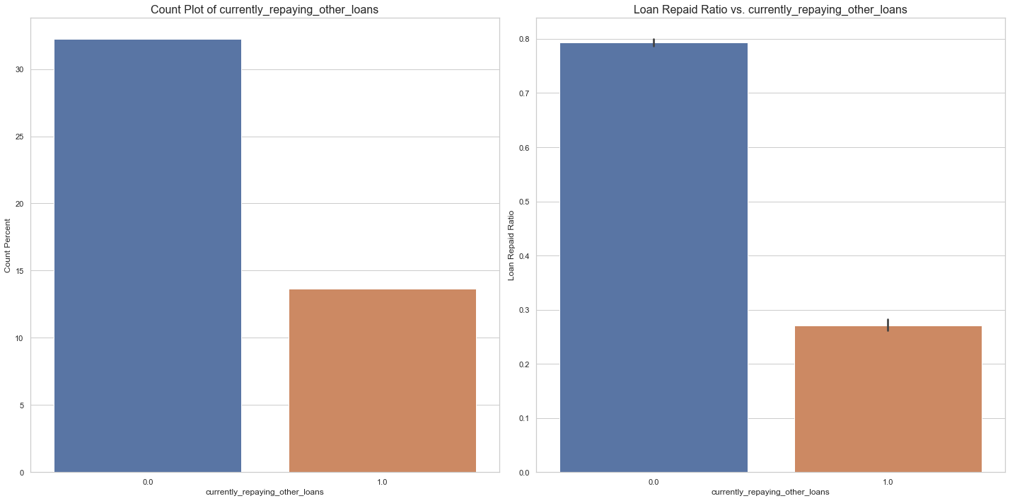
Loan Repayment Rate by other loans
Results:
- Around 14% loans were granted to borrowers who are currently paying other loans.
- Repayment Rate is less than 30% for those who are paying other loans.
#currently_repaying_other_loans
fig, ax = plt.subplots(nrows=1, ncols=2, figsize=(20, 10))
sns.barplot(x='currently_repaying_other_loans', y ='currently_repaying_other_loans',estimator=lambda x: len(x) / len(data) * 100, data=data, ax=ax[0])
ax[0].set_xlabel('currently_repaying_other_loans', fontsize=12)
ax[0].set_ylabel('Count Percent', fontsize=12)
ax[0].set_title('Count Plot of currently_repaying_other_loans', fontsize=16)

sns.barplot(x='currently_repaying_other_loans', y='loan_repaid', data=data, ax=ax[1])
ax[1].set_xlabel('currently_repaying_other_loans', fontsize=12)
ax[1].set_ylabel('Loan Repaid Ratio', fontsize=12)
ax[1].set_title('Loan Repaid Ratio vs. currently_repaying_other_loans', fontsize=16)
plt.tight_layout()
plt.show()
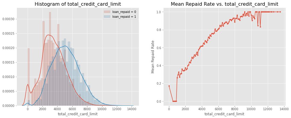
Loan Repayment Rate by Credit Card Limit
Results:
-
Borrowers who didn’t repay loan have credit card limit between $2000 to $6000, whereas the borrowers who did repay their loans had higher credit card limit ranging from $2000 to $10,000. These borrowers must be the ones with good credit scores.
-
Repayment rate increases as credit card limit increases. People approved for high credit limit must be the ones with good credit history so lesser chance of delinquency.
# Visualization of 'total_credit_card_limit'
grouped = data[['total_credit_card_limit', 'loan_repaid']].groupby('total_credit_card_limit')
grouped
mean = grouped.mean().reset_index()
mean
hist_kws={'histtype': 'bar', 'edgecolor':'black', 'alpha': 0.2}
fig, ax = plt.subplots(nrows=1, ncols=2, figsize=(16, 6))
sns.distplot(data[data['loan_repaid'] == 0]['total_credit_card_limit'],
             label='loan_repaid = 0', ax=ax[0], hist_kws=hist_kws)
sns.distplot(data[data['loan_repaid'] == 1]['total_credit_card_limit'],
             label='loan_repaid = 1', ax=ax[0], hist_kws=hist_kws)
ax[0].set_title('Histogram of total_credit_card_limit', fontsize=16)
ax[0].legend()
ax[1].plot(mean['total_credit_card_limit'], mean['loan_repaid'], '.-')
ax[1].set_title('Mean Repaid Rate vs. total_credit_card_limit', fontsize=16)
ax[1].set_xlabel('total_credit_card_limit')
ax[1].set_ylabel('Mean Repaid Rate')
ax[1].grid(True)
plt.show()
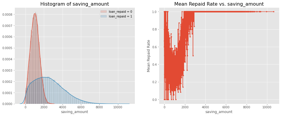
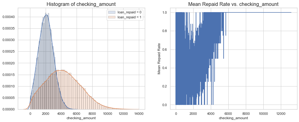
Loan Repayment Rate by Saving and Checking Amount
- Checking and Savings amount are important factors when deciding a borrower’s capacity to repay a loan.
- Borrowers who have lesser than ‘2000’ in savings and 4000 in checking are the ones who are more likely to default.
- Borrowers who have higher than 2000 in savings and anywhere from 2000 to 10,000 dollars in checking are the ones who have high repayment rate.
# Visualization of 'saving_amount'
grouped = data[['saving_amount', 'loan_repaid']].groupby('saving_amount')
grouped
mean = grouped.mean().reset_index()
mean
hist_kws={'histtype': 'bar', 'edgecolor':'black', 'alpha': 0.2}
fig, ax = plt.subplots(nrows=1, ncols=2, figsize=(16, 6))
sns.distplot(data[data['loan_repaid'] == 0]['saving_amount'],
             label='loan_repaid = 0', ax=ax[0], hist_kws=hist_kws)
sns.distplot(data[data['loan_repaid'] == 1]['saving_amount'],
             label='loan_repaid = 1', ax=ax[0], hist_kws=hist_kws)
ax[0].set_title('Histogram of saving_amount', fontsize=16)
ax[0].legend()
ax[1].plot(mean['saving_amount'], mean['loan_repaid'], '.-')
ax[1].set_title('Mean Repaid Rate vs. saving_amount', fontsize=16)
ax[1].set_xlabel('saving_amount')
ax[1].set_ylabel('Mean Repaid Rate')
ax[1].grid(True)
plt.show()
# Visualization of 'checking_amount'
grouped = data[['checking_amount', 'loan_repaid']].groupby('checking_amount')
grouped
mean = grouped.mean().reset_index()
mean
hist_kws={'histtype': 'bar', 'edgecolor':'black', 'alpha': 0.2}
fig, ax = plt.subplots(nrows=1, ncols=2, figsize=(16, 6))
sns.distplot(data[data['loan_repaid'] == 0]['checking_amount'],
             label='loan_repaid = 0', ax=ax[0], hist_kws=hist_kws)
sns.distplot(data[data['loan_repaid'] == 1]['checking_amount'],
             label='loan_repaid = 1', ax=ax[0], hist_kws=hist_kws)
ax[0].set_title('Histogram of checking_amount', fontsize=16)
ax[0].legend()
sns.lineplot(x= mean['checking_amount'], y= mean['loan_repaid'],ax = ax[1])
ax[1].set_title('Mean Repaid Rate vs. checking_amount', fontsize=16)
ax[1].set_xlabel('checking_amount')
ax[1].set_ylabel('Mean Repaid Rate')
ax[1].grid(True)
plt.show()
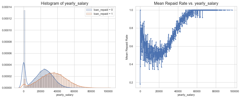
Loan Repayment Rate by Yearly Salary
Results:
- Borrowers who are unable to repay a loan earn less than 40,000 dollars a year
- Borrowers who earn more than 40,000 dollars a year have a repayment rate of more than 80%.
# Visualization of 'yearly_salry'
grouped = data[['yearly_salary', 'loan_repaid']].groupby('yearly_salary')
grouped
mean = grouped.mean().reset_index()
mean
hist_kws={'histtype': 'bar', 'edgecolor':'black', 'alpha': 0.2}
fig, ax = plt.subplots(nrows=1, ncols=2, figsize=(16, 6))
sns.distplot(data[data['loan_repaid'] == 0]['yearly_salary'],
             label='loan_repaid = 0', ax=ax[0], hist_kws=hist_kws)
sns.distplot(data[data['loan_repaid'] == 1]['yearly_salary'],
             label='loan_repaid = 1', ax=ax[0], hist_kws=hist_kws)
ax[0].set_title('Histogram of yearly_salary', fontsize=16)
ax[0].legend()
ax[1].plot(mean['yearly_salary'], mean['loan_repaid'], '.-')
ax[1].set_title('Mean Repaid Rate vs. yearly_salary', fontsize=16)
ax[1].set_xlabel('yearly_salary')
ax[1].set_ylabel('Mean Repaid Rate')
ax[1].grid(True)
plt.show()
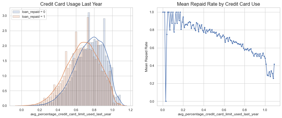
Loan Repayment by Last Year’s Credit Card Usage
Results:
- Borrowers unable to repay a loan have higher credit card usage than the ones who repay the loans.
- As the credit card usage increases, ability to repay a loan decreases.
not_null = data[~data['avg_percentage_credit_card_limit_used_last_year'].isnull()]
#avg_percentage_credit_card_limit_used_last_year

grouped = not_null[['avg_percentage_credit_card_limit_used_last_year', 'loan_repaid']].groupby('avg_percentage_credit_card_limit_used_last_year')
grouped
mean = grouped.mean().reset_index()
hist_kws={'histtype': 'bar', 'edgecolor':'black', 'alpha': 0.2}
fig, ax = plt.subplots(nrows=1, ncols=2, figsize=(16, 6))
sns.distplot(not_null[not_null['loan_repaid'] == 0]['avg_percentage_credit_card_limit_used_last_year'],
             label='loan_repaid = 0', ax=ax[0], hist_kws=hist_kws)
sns.distplot(data[data['loan_repaid'] == 1]['avg_percentage_credit_card_limit_used_last_year'],
             label='loan_repaid = 1', ax=ax[0], hist_kws=hist_kws)
ax[0].set_title('Credit Card Usage Last Year', fontsize=16)
ax[0].legend()
ax[1].plot(mean['avg_percentage_credit_card_limit_used_last_year'], mean['loan_repaid'], '.-')
ax[1].set_title('Mean Repaid Rate by Credit Card Use', fontsize=16)
ax[1].set_xlabel('avg_percentage_credit_card_limit_used_last_year')
ax[1].set_ylabel('Mean Repaid Rate')
ax[1].grid(True)
plt.show()
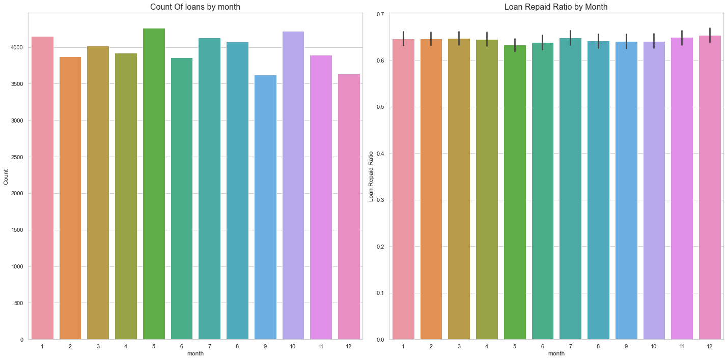
Repayment By Month
Results:
- A lot of loans are granted at the beginning of the year, in May and in October.
- Repayment rate remains almost the same across all the months.
fig, ax = plt.subplots(nrows=1, ncols=2, figsize=(20, 10))
sns.countplot(x='month', data=data, ax=ax[0])
ax[0].set_xlabel('month', fontsize=12)
ax[0].set_ylabel('Count', fontsize=12)
ax[0].set_title('Count Of loans by month', fontsize=16)

sns.barplot(x='month', y='loan_repaid', data=data, ax=ax[1])
ax[1].set_xlabel('month', fontsize=12)
ax[1].set_ylabel('Loan Repaid Ratio', fontsize=12)
ax[1].set_title('Loan Repaid Ratio by Month', fontsize=16)
plt.tight_layout()
plt.show()
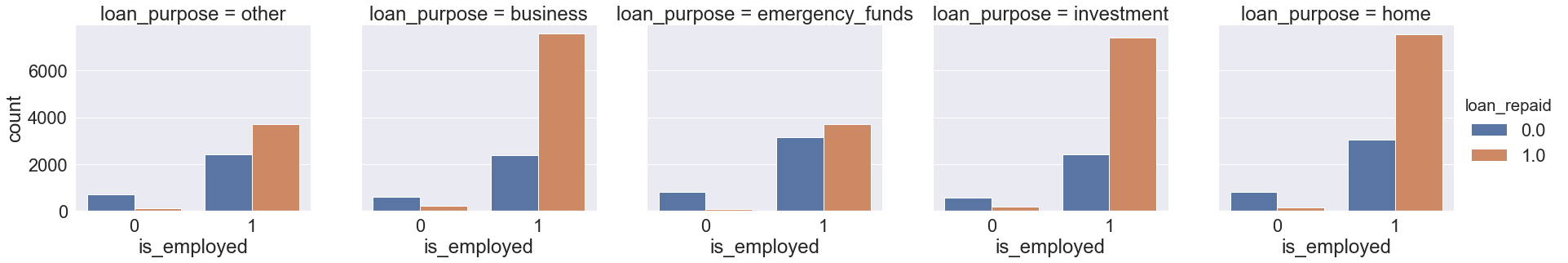
We can even look at the relationship of various variables together such as loan purpose by is_employed and loan_repaid. A lot of the borrowers who are unemployed apply for emergency loans.
sns.set_style('ticks')
sns.set(font_scale = 2)
sns.catplot("is_employed", col='loan_purpose', data=data, hue='loan_repaid', kind="count", col_wrap=5)
<seaborn.axisgrid.FacetGrid at 0x12980c4f0>
Feature Engineering
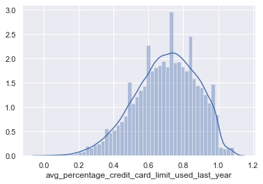
Avg_percentage_credit_card_limit
Avg_percentage_credit_card_limit_used_last_year is left-skewed which indicates that mean is lesser than the median so we will use median to impute the values
sns.set(font_scale = 1)
sns.distplot(data['avg_percentage_credit_card_limit_used_last_year'])
<matplotlib.axes._subplots.AxesSubplot at 0x12cddb6d0>
median_cc = data['avg_percentage_credit_card_limit_used_last_year'].median()
data = data.fillna({'avg_percentage_credit_card_limit_used_last_year':median_cc})
data.avg_percentage_credit_card_limit_used_last_year.isnull().sum()
0
#Rename avg_percentage_credit_card_limit_used_last_year to credit use
data.rename(columns={'avg_percentage_credit_card_limit_used_last_year':'credit_limit_used'},inplace=True)
is_first_loan, currently_repaying_loans, fully_repaid_previous_loans
We will create a new variable based on three columns: is_first_loan, currently_repaying_loans and fully_repaid_previous_loans :
Class 1: Not Repaid previous loan and currently paying other loans
Class 2: Paid previous loans and currently paying other loans
Class 3: First Loan
Class 4: Not paid previous loan and not paying other loans
Class 5: Repaid previous loan and not paying other loans
def new_variable(df):
    if((df['is_first_loan'] == 0) & (df['fully_repaid_previous_loans'] == 0) & (df['currently_repaying_other_loans'] == 1)):
        val = 1
    elif((df['is_first_loan'] == 0) & (df['fully_repaid_previous_loans'] == 1) & (df['currently_repaying_other_loans'] == 1)):
        val = 2
    elif((df['is_first_loan'] == 0) & (df['fully_repaid_previous_loans'] == 1) & (df['currently_repaying_other_loans'] == 0)):
        val = 5
    elif((df['is_first_loan'] == 0) & (df['fully_repaid_previous_loans'] == 0) & (df['currently_repaying_other_loans'] == 0)):
        val = 4
    else:
        val = 3
    return(pd.Series(val))
res = data.apply(new_variable,axis = 1)
data['prev_loan_status'] = res
data.loc[data.is_first_loan == 0,['is_first_loan','fully_repaid_previous_loans','currently_repaying_other_loans','prev_loan_status']]
| is_first_loan | fully_repaid_previous_loans | currently_repaying_other_loans | prev_loan_status | |
|---|---|---|---|---|
| 8 | 0 | 1.0 | 0.0 | 5 |
| 9 | 0 | 1.0 | 0.0 | 5 |
| 13 | 0 | 1.0 | 0.0 | 5 |
| 17 | 0 | 1.0 | 0.0 | 5 |
| 40 | 0 | 1.0 | 0.0 | 5 |
| ... | ... | ... | ... | ... |
| 101081 | 0 | 1.0 | 0.0 | 5 |
| 101083 | 0 | 1.0 | 1.0 | 2 |
| 101088 | 0 | 0.0 | 0.0 | 4 |
| 101090 | 0 | 1.0 | 0.0 | 5 |
| 101098 | 0 | 1.0 | 0.0 | 5 |
21865 rows × 4 columns
group_loan = data[['prev_loan_status','loan_repaid']].groupby('prev_loan_status').agg({'count','mean'}).reset_index()
group_loan.columns = group_loan.columns.droplevel(0)
group_loan.columns = ['prev_loan_status','total_count','repaid_rate']
group_loan['cnt_pct'] = 100* group_loan['total_count']/group_loan['total_count'].sum()
group_loan
| prev_loan_status | total_count | repaid_rate | cnt_pct | |
|---|---|---|---|---|
| 0 | 1 | 682 | 0.218475 | 1.431150 |
| 1 | 2 | 5828 | 0.277454 | 12.229823 |
| 2 | 3 | 25789 | 0.650006 | 54.117178 |
| 3 | 4 | 1450 | 0.751724 | 3.042767 |
| 4 | 5 | 13905 | 0.797339 | 29.179083 |
Class 5(previous loan fully paid and not paying other loans) has the highest repayment rate of 79%.
54% of the loans granted are First time loans and have repayment rate of 65%.
yearly salary and employment correlated
Unemployed borrowers will not have a salary to report so we will remove one of them
print(data[data['is_employed'] == 0]['yearly_salary'].unique())
[0]
One hot encoding for loan purpose
K unique values, only need K-1 features, so remove one redundant feature
data_cp = pd.get_dummies(data)
Remove redundant columns
X_new = data_cp.drop(columns = ['loan_id','date','loan_granted','is_first_loan','fully_repaid_previous_loans','currently_repaying_other_loans','is_employed','loan_purpose_other'],axis = 1)
X_new.head()
| total_credit_card_limit | credit_limit_used | saving_amount | checking_amount | yearly_salary | age | dependent_number | loan_repaid | month | week | dayofweek | prev_loan_status | loan_purpose_business | loan_purpose_emergency_funds | loan_purpose_home | loan_purpose_investment | |
|---|---|---|---|---|---|---|---|---|---|---|---|---|---|---|---|---|
| 2 | 6900 | 0.82 | 2085 | 3422 | 24500 | 38 | 8 | 1.0 | 7 | 29 | 0 | 3 | 0 | 0 | 0 | 0 |
| 5 | 6100 | 0.53 | 6163 | 5298 | 29500 | 24 | 1 | 1.0 | 11 | 45 | 2 | 3 | 0 | 0 | 0 | 0 |
| 7 | 4000 | 0.57 | 602 | 2757 | 31700 | 36 | 8 | 0.0 | 9 | 38 | 2 | 3 | 1 | 0 | 0 | 0 |
| 8 | 7000 | 0.52 | 2575 | 2917 | 58900 | 33 | 3 | 1.0 | 12 | 49 | 1 | 5 | 0 | 1 | 0 | 0 |
| 9 | 4300 | 0.83 | 722 | 892 | 5400 | 32 | 7 | 1.0 | 1 | 3 | 4 | 5 | 1 | 0 | 0 | 0 |
We have 16 features for model building
X_new.shape
(47654, 16)
LightGBM Model
LightGBM is a distributed and efficient gradient boosting framework that uses tree-based learning. It’s histogram-based and places continuous values into discrete bins, which leads to faster training and more efficient memory usage. In this piece, we’ll explore LightGBM in depth.
LightGBM Advantages
- Faster training speed and higher efficiency
- Lower memory usage
- Better accuracy
- Support of parallel and GPU learning
- Capable of handling large-scale data
- Is not affected by outliers and correlated variables
- Can handle categorical data
Train-Test Split
#Train test split
Y = X_new['loan_repaid']
Y.head()
2    1.0
5    1.0
7    0.0
8    1.0
9    1.0
Name: loan_repaid, dtype: float64
X = X_new.drop(columns= ['loan_repaid'],axis = 1)
X.shape
(47654, 15)
X_train, X_test, y_train, y_test = train_test_split(X, Y, test_size=0.25,random_state=42)
len(X_train),len(X_test),len(y_train),len(y_test)
(35740, 11914, 35740, 11914)
print(y_train.mean(),y_test.mean())
0.6450475657526581 0.6422695987913379
Prepare GBM Dataset and Tune Parameters
#create LightGBM dataset
d_train = lgb.Dataset(data=X_train, label=y_train,free_raw_data=False)
d_test = lgb.Dataset(data=X_test,label=y_test)
# Cross validation
#Using Default Values
params = {'learning_rate': 0.01,
          'boosting_type': 'gbdt',
          'objective': 'binary',
          'metric': ['binary_logloss', 'auc'],
          'sub_feature':0.8,
          'num_leaves': 31,
          'min_data': 20,
          'max_depth': 15,
          'is_unbalance': True}

history = lgb.cv(params, train_set=d_train, num_boost_round=1000, nfold=5,
                 early_stopping_rounds=10, seed=42, verbose_eval=False)
print('Best rounds:\t', len(history['binary_logloss-mean']))
Best rounds: 647
Prediction and Evaluation
# re-train the model and make predictions
clf = lgb.train(params, train_set=d_train, num_boost_round=647)
pred = clf.predict(X_test)
roc_auc = roc_auc_score(y_test,pred)
pred_int = (pred >=0.5).astype(int)
accuracy = accuracy_score(pred_int,y_test)
print('ROC score:{}, Accuracy at 0.5 threshold: {}'.format(roc_auc,accuracy))
ROC score:0.9774140994352406, Accuracy at 0.5 threshold: 0.9204297465167031
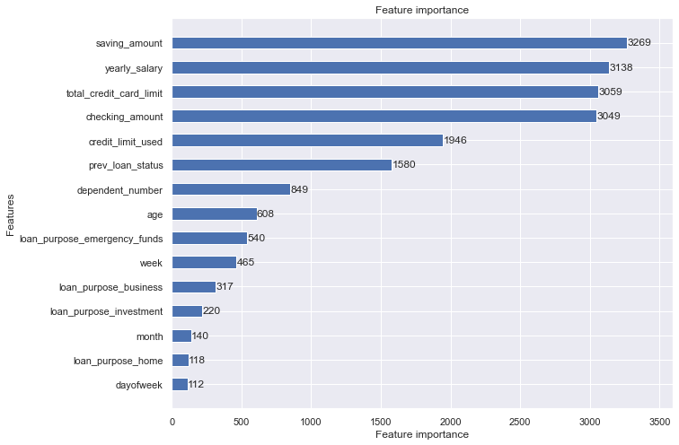
Feature Importance
Savings Amount, Yearly Salary, Total Credit Card Usage are among the top features that can help determine a borrower’s ability to repay a loan.
# feature importance
features = clf.feature_name()
importance = clf.feature_importance()

fig, ax = plt.subplots(figsize=(10, 8))
lgb.plot_importance(clf, ax=ax, height=0.5)
plt.show()
Bank Profit Calculation
We will assume if the loan is repaid then bank earns a $1 and if the loan is not repaid then a loss of -1.
Bank profit by old model
#Total Profit from original Bank model

loan_paid = y_test.astype(int).values

bank_profit = np.sum(loan_paid * 2 - 1)
print('Bank profit:\t', bank_profit)
Bank profit: 3390
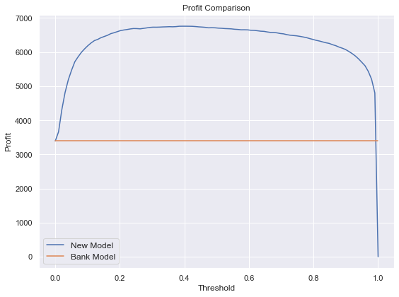
Bank profit by New Model at different thresholds
We will calculate the profit at different thresholds and choose the one where we get maximum profit
# Calculate profit according to different thresholds
def calc_threshold(loan_paid,probability,threshold):
    loan_granted = (probability > threshold).astype(int)
    profit = 0
    for i in range(len(loan_paid)):
        if loan_granted[i] == 1:
            if loan_paid[i] == 0:
                profit -= 1
            else:
                profit += 1

    return profit
# calculate the profit according to given threshold
thresholds = list(np.linspace(0, 1, 100))
profits = []

for threshold in thresholds:
    profits.append(calc_threshold(loan_paid, pred, threshold))
thresh_prof = pd.DataFrame({'threshold':thresholds,'profit':profits})
thresh_prof.loc[thresh_prof.profit.argmax(),:]
threshold       0.393939
profit       6756.000000
Name: 39, dtype: float64
With the new model, bank can make a profit of 6756 dollars which is double of the bank’s earlier profit of 3390.
fig, ax = plt.subplots(figsize=(8, 6))
ax.plot(thresholds, profits, label='New Model')
ax.plot(thresholds, [bank_profit] * len(thresholds), label='Bank Model')
ax.set_xlabel('Threshold', fontsize=12)
ax.set_ylabel('Profit', fontsize=12)
ax.set_title('Profit Comparison')
ax.legend(fontsize=12)
plt.tight_layout()
plt.show()
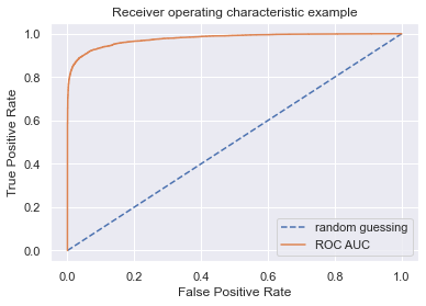
fpr,tpr,threshold = roc_curve(loan_paid, pred)
print("Area under the Receiver Operating Characteristic Curves (ROC AUC) is %f "
      %(roc_auc_score(loan_paid, pred)))
Area under the Receiver Operating Characteristic Curves (ROC AUC) is 0.977414
plt.figure()
plt.plot([0,1],[0,1], linestyle = '--', label = 'random guessing')
plt.plot(fpr, tpr, label = "ROC AUC" )
plt.xlabel('False Positive Rate')
plt.ylabel('True Positive Rate')
plt.title('Receiver operating characteristic example')
plt.legend(loc='lower right')
<matplotlib.legend.Legend at 0x137690a30>
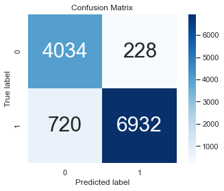
Classification Report at 0.5 threshold
False Positives: If the model predicts that a loan will be repaid and the borrower defaults, then bank will lose money. We would like to keep our false positives low.
False Negatives: If the model predicts that a loan will not be repaid but the borrower does repay, the bank might lose a potential customer by not granting a loan. In this case loss is going to be 0.
More than False negatives, we should focus on high precision and keeping the false positives low.
print(classification_report(y_true = y_test, y_pred=pred_int))
              precision    recall  f1-score   support

         0.0       0.85      0.95      0.89      4262
         1.0       0.97      0.91      0.94      7652

    accuracy                           0.92     11914
   macro avg       0.91      0.93      0.92     11914
weighted avg       0.93      0.92      0.92     11914
cm = confusion_matrix(y_test, pred_int)

# view with a heatmap
sns.heatmap(cm, annot=True, annot_kws={"size":30}, cmap='Blues', square=True, fmt='.0f')
plt.ylabel('True label')
plt.xlabel('Predicted label')
plt.title('Confusion Matrix')
Text(0.5, 1.0, 'Confusion Matrix')
Precision and Recall at 0.4 threshold
We can see that the true positive predictive power i.e model predicts that a borrower will reapy and borrower did repay increased at the new threshold.
pred_int_new = (pred >= 0.39).astype(int)
accuracy_score(y_test,pred_int_new)
0.9247104247104247
print(classification_report(y_true = y_test, y_pred=pred_int_new))
              precision    recall  f1-score   support

         0.0       0.87      0.92      0.90      4262
         1.0       0.96      0.93      0.94      7652

    accuracy                           0.92     11914
   macro avg       0.91      0.92      0.92     11914
weighted avg       0.93      0.92      0.93     11914
cm = confusion_matrix(y_test, pred_int_new)

# view with a heatmap
sns.heatmap(cm, annot=True, annot_kws={"size":30}, cmap='Blues', square=True, fmt='.0f')
plt.ylabel('True label')
plt.xlabel('Predicted label')
plt.title('Confusion Matrix at new threshold')
Text(0.5, 1.0, 'Confusion Matrix at new threshold')
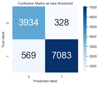
Strategy for Denied Application
My model is able to predict 7083 loans will be repaid and they did. The true positive predictive accuracy is 91.1 %. Thus, if we grant a loan to a previously denied application then the bank can make a lot of profit.
pos_ind = (pred_int_new == 1)

tpr_new = np.sum(y_test[pos_ind] == 1) # number of loan repaid
print("number of cases that model predicts repay and repaid: {}".format(tpr_new))

fpr_new = np.sum(y_test[pos_ind] == 0) # number of loan defaulted
print("number of cases that model predicts repay but defaulted: {}".format(fpr_new))

tot = (np.sum(y_test[pos_ind] == 1) - np.sum(y_test[pos_ind] == 0))/sum(pos_ind)
print("score to gain when granting a loan: {}".format(tot))
number of cases that model predicts repay and repaid: 7083
number of cases that model predicts repay but defaulted: 328
score to gain when granting a loan: 0.9114829307785723
Impact Analysis of “is_employed”
Results:
- There are 1047 unemployed borrowers and 10,867 employed borrowers in the dataset
- If an applicant is unemployed, then our model predicts 14% of the loans will be repaid and grants them the loan. If an applicant is employed, then model predicts 67% of the loans will be repaid and grants them the loan.
- Among the ones who are unemployed and model predicts to grant the loan, 94.4% repay the loans.
- Among the ones who are employed and model predicts to grant the loan, 95.5% do repay the loans.
unemployed = len(X_test[X_test['yearly_salary'] == 0])
not_emp = len(X_test) - unemployed
print('Number of unemployed borrowers in the test set : {}\nNumber of employed borrowers : {}'.format(unemployed,not_emp))
Number of unemployed borrowers in the test set : 1047
Number of employed borrowers : 10867
loan_grant_unemp = pred_int_new[X_test['yearly_salary'] == 0].mean()
loan_grant_emp = pred_int_new[X_test['yearly_salary'] != 0].mean()
print('Loan Grant Rate for unemployed by the model : {}\nLoan Grant Rate for employed by the model:{}'.format(loan_grant_unemp,loan_grant_emp))
Loan Grant Rate for unemployed by the model : 0.13753581661891118
Loan Grant Rate for employed by the model:0.6687218183491304
#Repay rate for unemployed
unemployed_granted_ind = np.logical_and(X_test['yearly_salary']==0,pred_int_new==1)
unemp_repay = y_test[unemployed_granted_ind].mean()
0.9444444444444444
#Repay rate for employed
employed_granted_ind = np.logical_and(X_test['yearly_salary']!=0,pred_int_new==1)
emp_repay = y_test[employed_granted_ind].mean()
emp_repay
0.9559653226916196
Savings Amount
pred_int_new[X_test['saving_amount'] < 4000].mean()
0.5704473910140228
pred_int_new[X_test['saving_amount'] >= 4000].mean()
1.0
Recommendations:
-
According to the feature importance plot, the most important feature is ‘savings amount’. This makes perfect sense because if a person has money in the savings account, it is more likely that he/she will be able to repay the loan. Given the data, our model predicts 100% repayment if savings amount exceeds 4000 dollars
-
Borrower’s employment status is very important. If a person is employed it is highly likely that he/she will be able to repay the loan. Target customers who are employed and have a yearly salary of atleast 60,000. This will reduce the probability of default.
-
Number of dependents does affect the repayment rate to some extent. Bank should modify it’s strategy to reduce giving loans to people with 8 dependents and give more loans to people with less dependents
-
Borrowers who have high credit card limit could mean they have good financial standing to be approved for such limits. These users have higher chance of repaying the loans. Hence, they could be granted a loan.
-
The gradient boosted model developed should be implemented and loans should be given to the ones predicted to have high repayment probability. This model has 92% positive predictive power and provides double the profit the bank is currently making.